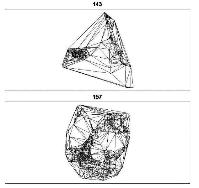
Now we are going to get into another class of home range estimators that use polygons created by Delaunay triangulation of a set of relocations and then removing a subset of the resulting triangles. These polygons can have concave edges, be composed of disjoint regions, and contain empty portions of unused space within hull interiors. This estimator has been described in the adehabitatHR package and evaluated on black-footed albatross (Phoebastria nigripes; Downs and Horner 2009). Polygon-based estimators may be a useful method for a variety of species but research has been limited.
- Exercise 4.7 - Download and extract zip folder into your preferred location
- Set working directory to the extracted folder in R under File - Change dir...
-
First we need to load the packages needed for the exercise
library(adehabitatHR)
library(maptools) - Now open the script "CHPscript.R" and run code directly from the script
- Now read in the locations and create a Spatial Points Data Frame for the 2 animals by ID using the code that follows:
twocats <-read.csv("pantherjitter.csv",
header=T)
data.xy = twocats[c("X","Y")] - Creates a class of Spatial Points for all locations with projection defined
data.xy = twocats[c("x","y")]
xysp <- SpatialPoints(data.xy)
proj4string(xysp) <- CRS("+proj=utm +zone=17N +ellps=WGS84") - Creates a Spatial Data Frame from Spatial points
sppt<-data.frame(xysp) - Creates a spatial data frame of ID
idsp<-data.frame(twocats[1]) - Merges ID and Date into the same spatial data frame
coordinates(idsp)<-sppt
head(as.data.frame(idsp))
#Results from the above code
ID X Y
1 121 494155.6 2904240
2 121 498182.3 2905598
3 121 498476.2 2905114
4 121 499210.5 2905661
5 121 499467.3 2905533
6 121 502960.9 2904391 - Code for estimation of home range using CharHull from adehabitatHR
res <- CharHull(idsp[,1])
class("res") - Code to display the home range in R (Fig. 4.14).
plot(res)
Figure 4.14. Example of CHP home range for 2 Florida panther - Code to compute the home range size for 20−100 percent
MCHu2hrsize(res)
20 10.70262 150.2998
30 28.73158 342.9798
40 79.15079 688.7553
50 172.95317 1418.7588
60 343.12024 2319.157870 700.94072 3574.5525
OR
80 1333.94110 5910.8221
90 2431.27046 12912.0320
100 5538.22402 103361.1336 - Computes the home range size for 95 percent
MCHu2hrsize(res, percent=95)
OR use
getverticeshr(res, percent=95)
Number of SpatialPolygons: 2
Variables measured:
Keep in mind that CHP estimates in Figure 4.14 are for 20−100 percent with 100% filling in the entire area traversed by each animal. If you want to visualize core area (i.e., 50%) or 95% that are commonly reported, the resulting home ranges might be more appropriate visualization of the area an animal traverses.
id area
1 121 2413.518
2 143 12845.298

