1.10 Creating buffers

For this exercise, we will again be working with the Colorado mule deer locations and rasters from earlier sections (1.3, 1.7). Creating buffers around locations of animals, plots, or some
other variable may be necessary to determine what occurs around the locations. Often times,
in resource selection studies, we may want to generate buffers that can be considered used
habitat within the buffer as opposed to simply counting only the habitat that the location is
in. Let's begin with loading the proper packages and mule deer locations from previous
exercise. Because we are dealing with the raster layer projected in Albers, we will need to
project our mule deer locations as we did above.

1. Exercise 1.10 - Download and extract zip folder into your preferred location
2. Set working directory to the extracted folder in R under File - Change dir...
3. First we need to load the packages needed for the exercise
   library(sp)
   library(lattice)
   library(rgdal)
   library(rgeos)
   library(raster)
4. Now open the script "BufferScript.R" and run code directly from the script
   
   muleys <-read.csv("muleysexample.csv", header=T)
   summary(muleys$id)
   
   #Let's subset data so there are fewer locations to work with
   muley8 <- subset(muleys, id=="D8")
   str(muley8)
   summary <- table(muley8$UTM_Zone,muley8$id)
   summary(muley8$id)
   muley8$id <- factor(muley8$id)
   
   #Remove outlier locations if needed
   summary(muley8$Long)
   # Min. 1st Qu. Median Mean 3rd Qu. Max.
   # -111.8 -108.9 -108.9 -108.9 -108.9 -108.8
   #NOTE: Min. of -111.8 is an outlier so remove
   summary(muley8$Lat)
   # Min. 1st Qu. Median Mean 3rd Qu. Max.
   # 33.38 37.84 37.84 37.83 37.85 37.86
   #NOTE: Min. of 33.38 is an outlier so remove
   newmuley8 <-subset(muley8, muley8$Long > -111.7 & muley8$Lat > 37.80)
   str(newmuley8)
   muley8 <- newmuley8
   
   #Make a spatial data frame of locations after removing outliers
   coords<-data.frame(x = muley8$Long, y = muley8$Lat)
   crs<-"+proj=longlat +datum=WGS84 +no_defs +ellps=WGS84 +towgs84=0,0,0"
   head(coords)
   
   deer.spdf <- SpatialPointsDataFrame(coords= coords, data = muley8, proj4string =
   CRS(crs))
   head(deer.spdf)
   class(deer.spdf)
   proj4string(deer.spdf)
   
   #Again let's project the deer.spdf to Albers
   Albers.crs <-CRS("+proj=aea +lat_1=29.5 +lat_2=45.5 +lat_0=23
   +lon_0=-96 +x_0=0 +y_0=0 +ellps=GRS80 +towgs84=0,0,0,0,0,0,0+units=m
   +no_defs")
   deer.albers <-spTransform(deer.spdf, CRS=Albers.crs)
   class(deer.albers)
   proj4string(deer.albers)
   head(deer.spdf)
   head(deer.albers)
5. Clip the study.zoom so we can zoom in on mule deer 8 locations as we did in previous exercise but with a bounding box of only mule deer 8 locations.
   
   bbox(deer.albers)
   bb1 <- cbind(x=c(-1115562,-1115562,-1120488,-1120488, -1115562),
   y=c(1718097,1722611,1722611,1718097,1718097))
   AlbersSP <- SpatialPolygons(list(Polygons(list(Polygon(bb1)),"1")),
   proj4string=CRS(proj4string(deer.albers)))
   plot(AlbersSP)
   points(deer.albers, col="red")
6. Load the vegetation raster layer textfile clipped in ArcMap to be within several counties around the mule deer locations. Plot the points and bounding box over the vegetation layer and notice they are barely visible due to the large extent of the raster layer.
   
   veg <-raster("extentnlcd2.txt")
   plot(veg)
   plot(AlbersSP,add=T)
   points(deer.albers, col="red")
7. We can clip the vegetation raster and plot the bounding box polygon and locations on the raster. Notice that the locations are nearly off the extent of the raster.
   
   bbclip <- crop(veg, AlbersSP)
   plot(bbclip)
   plot(AlbersSP,add=T,)
   points(deer.albers, col="red")
8. So let's create a new bounding box that encompass mule deer 8 locaitons but also extends beyond the periphery of the outermost locations. Then clip the large vegetation raster again so it is within the newly created bounding box polygon.
   
   bbox(deer.spdf)
   bb1 <- cbind(x=c(-1115000,-1115000,-1121000,-1121000, -1115000),
   y=c(1717000,1723000,1723000,1717000,1717000))
   AlbersSP <- SpatialPolygons(list(Polygons(list(Polygon(bb1)),"1")),
   proj4string=CRS(proj4string(deer.albers)))
   
   #Clip the vegetation raster within the boundaries of the new "AlbersSP."
   bbclip <- crop(veg, AlbersSP)
   windows()
   
   #Plot the clipped raster, bounding polygon, and mule deer 8 locations
   plot(bbclip)
   plot(AlbersSP,lwd=2,add=T)
   points(deer.albers, col="red")
9. To conduct some analyses, let's create 100 m buffered circles around all the locations and extract vegetation that occurs in each buffered circle.
   
   extract(bbclip,deer.albers)
   settbuff=gBuffer(deer.albers,width=100)
   plot(bbclip)
   plot(settbuff, add=TRUE, lty=2)
   table(extract(bbclip,settbuff))
   
   #Cell size of raster layer
   res(bbclip)
   30^2 #30 x 30 m resolution of the raster
   [1] 900
   > 900*37 #Times the number of cells in category 21 (i.e., developed habitat)
   [1] 33300
   > (900*37)/1000000 #Divide to convert square meters to square kilometers
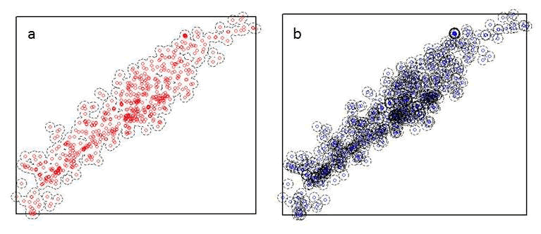
   0.0333 km2 #habitat 21
10. Most efforts will want percent habitat or area of each habitat defined individually for each location (i.e., within each buffered circle). To do this we only need to specify in the gBuffer function to create unique buffered circles with the byid=TRUE command (Fig. 1.9a,b).

Figure 1.9: Buffers around mule deer locations using the a) byid=FALSE (default) and b) byid=TRUE for the gBuffer function using package rgeos.

settbuff=gBuffer(deer.albers, width=100, byid=TRUE)
windows()
plot(bbclip)
points(deer.albers, col="blue")
plot(settbuff, add=TRUE, lty=2)

#Extract the amount of vegetation in each buffer and place it in a table by
buffer ID
e= extract(bbclip,settbuff)
et=lapply(e,table)
et

#Example below identifies buffered circles number 328
et[[328]]#Buffer ID 328 has 3 vegetation categories 41, 42, and 52 of 4, 7, and 24 cells, respectively

41 42 52
4 7 24