- Exercise 6.2 - Download and extract zip folder into your preferred location
- Set working directory to the extracted folder in R under File - Change dir...
- First we need to load the packages needed for the exercise
library(rasterVis)
library(raster)
library(rgl) -
Now open the script "DEMscript.R" and run code directly from the script
dem <-raster("dcdemascii12.txt")
plot(dem)
#Or as a .tif file seems to look better
dem2 <- raster("dovecreekdem.tif")
plot(dem2)
if (require(rgl)) {
extent(dem2) <- c(0, 610, 0, 870)
drape <- cut(dem, 5)
plot3D(dem2, drape=drape, zfac=2)
}
#or simply
plot3D(dem2,drape=dem2) - We can also create a variety of covariates using DEMs (i.e., slope, aspect)
highGround = dem > 2000
slope = terrain(dem,opt='slope', unit='degrees')
aspect = terrain(dem,opt='aspect',unit='degrees')
hill = hillShade(slope,aspect,40,270)
plot(hill,col=grey(0:100/100),legend=FALSE)
plot(dem2,col=rainbow(25,alpha=0.35))
windows()
plot(slope,col=rainbow(25,alpha=0.35))
windows()
plot(aspect,col=rainbow(25,alpha=0.35)) - We can also investigate various components of the ruggedness of terrain in a DEM with the function terrain in the raster package. TRI (Terrain Ruggedness Index) is the mean of the absolute differences between the value of a cell and the value of its 8 surrounding cells. Values of TRI are lower in flatter areas but high in both steep areas and in steep, rugged areas (Sappington et al. 2007). TPI (Topographic Position Index) is the difference between the value of a cell and the mean value of its 8 surrounding cells. Topographic position (e.g., valley bottom, mid-slope, ridge-top) can provide valuable information about the geomorphology of the region (Skidmore 1990). Roughness is the difference between the maximum and the minimum value of a cell and its 8 surrounding cells. Roughness is the difference between the maximum and the minimum value of a cell and its 8 surrounding cells.
x <- terrain(dem2, opt=c('slope', 'aspect'), unit='degrees')
plot(x)
# TPI for different neighborhood size:
tpiw <- function(x, w=5) {
m <- matrix(1/(w^2-1), nc=w, nr=w)
m[ceiling(0.5 * length(m))] <- 0
f <- focal(x, m)
x - f
}
tpi5 <- tpiw(dem2, w=5)
tpi = terrain(dem,opt='tpi')
summary(tpi)
plot3D(tpi)
tri = terrain(dem,opt='tri')
summary(tri)
plot3D(tri)
ruf = terrain(dem,opt='roughness')
plot3D(ruf)
#Load vegetation raster layer textfile clipped in ArcMap
#crop <-raster("crop2012utm.txt")
crop <-raster("crop2012utm12.tif")
plot(crop)
class(crop)
as.matrix(table(values(crop)))
proj4string(crop)
plot3D(dem,drape=crop)
crop
# reclassify the values into 9 groups if needed
# all values between 0 and 20 equal 1, etc.
m <- c(-Inf,0,NA,2, 7, 2, 20, 60, 3, 60, 70, 4, 110, 132, 5, 133, 150, 6, 151, 172, 7, rclmat <- matrix(m, ncol=3, byrow=TRUE)
rc <- reclassify(crop, rclmat)
plot(rc)
rc
plot3D(dem2,drape=rc)
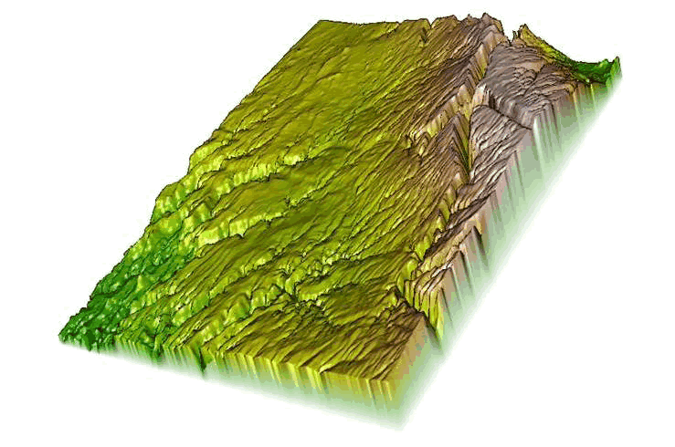
Figure 6.2: Example of a Digital Elevation Model in 3D using rasterVis package in R.

