- Exercise 1.7 - Download and extract zip folder into your preferred location
- Set working directory to the extracted folder in R under File - Change dir...
- First we need to load packages to work with raster datasets
install.packages(c("adehabitat","adehabitatHR","maptools","raster", "rgdal"))
library(rgdal)
library(raster)
library(adehabitat)
library(adehabitatHR)
library(maptools) -
Now open the script "RasterScript.R" in that folder and run code directly from the script. Create an Ascii file from your raster grid in ArcMap 10.X if experimenting with your own raster using the following Toolbox in ArcMap 10.X:
ArcToolbox - Conversion Tools - From Raster - Raster to Ascii
-
Alternatively, you can set your working directory by opening a previously saved workspace by double clicking it in that folder which will also serve to set that folder as the working directory. All of the raster layers we are going to use will be located here
#Note: Most of the exercises that follow are exploratory in nature and not the recommended way to bring raster data into R. I include these exercises only for those that may perhaps only have alternate rasters available (e.g., ASCII). I would recommend using .tif and not ASCII or .txt files as in the first few exercises below. -
If you have troubles getting a raster to Ascii in ArcMap to actually show up as an Ascii file there is good reason. We need to rename the text file by replacing ".txt" with ".asc" in Windows Explorer. ArcMap will not save as an ".asc" file and I have no idea why!
- Here is some code to import Ascii files (i.e., rasters) from ArcMap into R using one of several packages. Ascii files can be categorical (Vegetation/Habitat categories) or numeric (DEMs).
#Import raster as text using the "raster" package
library(rgdal)
library(raster)
r <-raster("polyascii2.txt")
proj4string(r)#Note: No projection information was imported with the raster
plot(r)
#Assign projection information for imported text file
## Path of the file to be imported
proj4string(r) <-CRS("+proj=aea +lat_1=29.5 +lat_2=45.5 +lat_0=23
+lon_0=-96 +x_0=0 +y_0=0 +ellps=GRS80 +towgs84=0,0,0,0,0,0,0 +units=m +no_defs")
r; proj4string(r) ##Or import raster as an Ascii files (factor) using "adehabitat" package for file1, file2, and file3 in the 3 sections of code below:
file1 <- paste("polyextract2.asc", sep = "\\")
levelfile <- paste("TableExtract.txt", sep = "\\")
asp <- import.asc(file1, lev = levelfile, )
image(asp)
asp
str(asp)
NOTE: "Levelfile" refers to a text file created from exporting the raster
#Now let's look at the vegetation categories of the file
value attribute table from ArcMap by opening in table of contents and
exporting as a text file
ta <- table(as.vector(asp))
names(ta) <- levels(asp)[as.numeric(names(ta))]
ta
file2 <- paste("polyclip.asc", sep = "\\")
levelfile2 <- paste("TableClip.txt", sep = "\\")
asp2 <- import.asc(file2, lev = levelfile2, )
image(asp2)
asp2
str(asp2)
#Shows 7 vegetation categories
#Now let's look at the vegetation categories of the file
ta2 <- table(as.vector(asp2))
names(ta2) <- levels(asp2)[as.numeric(names(ta2))]
ta2 - R won't recognize double digit veg categories with this method so reclassify in ArcMap then import raster as an Ascii files (factor) using:
file3 <- paste(polyascii2.asc")
levelfile3 <- paste("TableCode.txt")
asp3 <- import.asc(file3, lev = levelfile3, )
image(asp3)
asp3
str(asp3)
NOTE: "Levelfile" refers to a text file created from exporting the raster value attribute table from ArcMap by opening in table of contents and exporting as a text file and then edited to look like this:
"VALUE","COUNT","VEGCLASS"
1,464368,DEVELOPED
2,186853,FOREST
3,185059,SHRUB
4,509415,GRASS
5,341023,CROP
6,251492,WET
7,350491,NON
#Using "asp" results in the following:
Raster map of class "asc": Cell size: 30 Number of rows: 3245
Number of columns: 3353 Type: factor
#Now let's look at the vegetation categories of the file
ta3 <- table(as.vector(asp3))
names(ta3) <- levels(asp3)[as.numeric(names(ta3))]
ta3 - Or import raster as an Ascii files (numeric like a DEM) using:
fileElev <- paste("demascii.asc", sep = "\\"))
elev <- import.asc(fileElev)
image(elev)
plot(elev, col=terrain.colors(10))
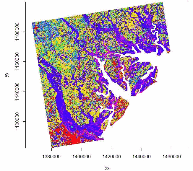
Figure 1.7: Imported raster dataset showing coastline and tributaries.
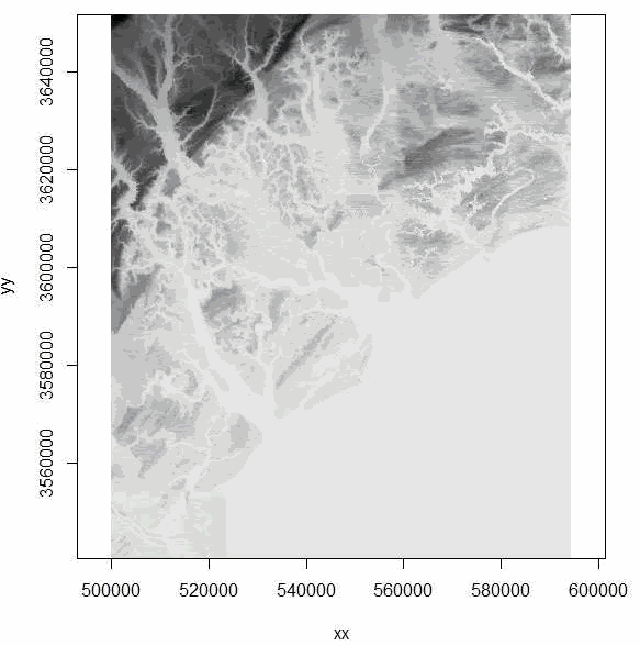
Figure 1.8: Imported Digital Elevation Model using adehabitat package showing coastline and tributaries. - We can also use the "rgdal" package to import an ascii grid as a Spatial Grid Data Frame
habitat <- readGDAL("polyascii2.asc")
proj4string(habitat) <-CRS("+proj=aea +lat_1=29.5 +lat_2=45.5 +lat_0=23 +lon_0=-96 +x_0=0 +y_0=0 +datum=NAD83 +units=m +no_defs +ellps=GRS80 +towgs84=0,0,0")
image(habitat)
str(habitat) - Now let's add some shapefiles to our raster
#Load county shapefile
county<-readOGR(dsn=".",layer="BeaufortCoAlbers")
proj4string(county)
spplot(county)
polys <- as(county, "SpatialPolygons")
plot(polys,add=T,lwd=2)
polys
text(coordinates(polys), labels="Beaufort")
proj4string(polys)
#Load airport runway shapefile
run<-readOGR(dsn=".",layer="RunwayAlbers")
proj4string(run)
spplot(run)
polys2 <- as(run, "SpatialPolygons")
plot(polys2,add=T,lwd=2)
polys2
proj4string(polys2)
#Load aircraft flight pattern shapefile
path<-readOGR(dsn=".",layer="FlightImage")
proj4string(path)
spplot(path)
polys3 <- as(path, "SpatialLines")
plot(polys3,add=T,lty="32", col="blue")
polys3
proj4string(polys3)
#Load roads shapefile for Beaufort County
road<-readOGR(dsn=".",layer="CountyRoadAlbers")
proj4string(road)
#spplot(road)
polys4 <- as(road, "SpatialLines")
plot(polys4,add=T,lty="22", col="green")
polys4
proj4string(polys4) - Plot out all the shapefiles overlayed on each other with and without the raster.
plot(county)
plot(road, add=T)
plot(run, col="red",add=T)
plot(path, col="blue",add=T) - Clip the raster within the county polygon for a zoomed in view then plot
#Clip using the raster imported with "raster" package
clip <- crop(r, polys)
plot(clip)
plot(polys,add=T,lwd=2)
plot(polys2,add=T,lwd=2, col="red")
plot(polys3,add=T,lty="62", col="blue")
plot(polys4,add=T,lty="22", col="green") - Let's reclassify layer to get fewer vegetation categories to make raster easier to work
with.
#Load vegetation layer
veg <-raster("polydouble.txt")
plot(veg)
veg
# Reclassify the values into 7 groups with all values between 0 and 20 equal
# 1, 21 to 40 equal 2, etc.
m <- c(0, 19, 1, 20, 39, 2, 40, 50, 3, 51,68, 4, 69, 79, 5, 80, 88, 6, 89, 99, 7)
rclmat <- matrix(m, ncol=3, byrow=TRUE)
rc <- reclassify(veg, rclmat)
plot(rc)
rc
#Now, let's remove water that is coded 11 and No Data that is coded as 127
m <- c(0, 19, NA, 20, 39, 1, 40, 50, 2, 51,68, 3, 69,79, 4, 80, 88, 5, 89, 99, 6, 100, 150, NA)
rclmat1 <- matrix(m, ncol=3, byrow=TRUE)
rc1 <- reclassify(veg, rclmat1)
plot(rc1)
rc1 - We can load some vulture locations to extract landcover that each location occurs in that will be considered "used" habitat in resource selection analysis.
#Import bird 49 locations to R
bv49 <-read.csv("Bird49.csv", header=T)
str(bv49)#How many bird locations?
#Make a spatial data frame of locations and convert to Albers
coords<-data.frame(x = bv49$x, y = bv49$y)
crs<-"+proj=utm +zone=17N +ellps=WGS84"
coords
bvspdf <- SpatialPointsDataFrame(coords= coords, data = bv49, proj4string = CRS(crs))
str(bvspdf)
bvspdf[1:5,]
points(bvspdf, col="red")
bv49Albers <-spTransform(bvspdf, CRS("+proj=aea +lat_1=29.5 +lat_2=45.5 +lat_0=23 +lon_0=-96 +x_0=0 +y_0=0 +ellps=GRS80 +towgs84=0,0,0,0,0,0,0 +units=m +no_defs"))
class(bv49Albers)
proj4string(bv49Albers)
bv49Albers[1:5,]
points(bv49Albers, col="red")
#Determine which of those points lie within a cell that contains data by using the extract function. The extract function will extract covariate information from the raster at a particular point.
veg.survey<-extract(veg, bv49Albers)
veg.survey
veg.survey<-subset(bv49Albers,!is.na(veg.survey))
plot(veg.survey, col="black", add=T) - We can also create some random points within the extent of the area to be considered as "available" habitat.
#First we need to create a grid across the study site with sample points
Sample.points<-expand.grid(seq(veg@extent@xmin, veg@extent@xmax, by=1000), weight = seq(veg@extent@ymin, veg@extent@ymax, by=1000))
points(Sample.points, bg="red", cex=.5,col="red")
#Now create some random points using the minimum and maximum coordinates of the raster to determine the range of points from which to select x and y
x.pts<-sample(seq(veg@extent@xmin, veg@extent@xmax, by=10),1000) ##generate
#x coordinates for random points
y.pts<-sample(seq(veg@extent@ymin, veg@extent@ymax, by=10),1000)
#Now create a spatial points file from the randomly generated points
coords2<-data.frame(x = x.pts, y = y.pts)
crs2<-"+proj=aea +lat_1=29.5 +lat_2=45.5 +lat_0=23 +lon_0=-96 +x_0=0 +y_0=0 +ellps=GRS80 +towgs84=0,0,0,0,0,0,0 +units=m +no_defs"
coords2
points(coords2, bg="red", cex=.5,col="blue")
#Determine which of those points lie within a cell that contains data by using the extract function. The extract function will extract covariate information from the raster at a particular point.
veg.sample<-extract(veg, sample.pts)
veg.sample
veg.sample<-subset(sample.pts,!is.na(veg.sample))
str(veg.sample)
points(veg.sample, col="green") - We can also do the same using the clipped vegetation raster to be more in line with vulture locations or using the reclassified vegetation categories. For each locations, we can determine if a locations lies within a cell that contains data by using the extract function and this will extract covariate information from the raster at a each location.
clip.survey<-extract(clip, bv49Albers)
clip.survey
clip.survey<-subset(bv49Albers,!is.na(clip.survey))
plot(clip.survey, col="black", add=T)
#Create a regular grid and do the same thing
Sample.points2<-expand.grid(seq(clip@extent@xmin, clip@extent@xmax, by=1500), weight = seq(clip@extent@ymin, clip@extent@ymax, by=1500))
points(Sample.points2, bg="red", cex=.5,col="red")
#Create random points using the minimum and maximum coordinates of the raster
x.pts2<-sample(seq(clip@extent@xmin, clip@extent@xmax, by=10),500)
y.pts2<-sample(seq(clip@extent@ymin, clip@extent@ymax, by=10),500)
#Now create a spatial points file from the randomly generated points
coords3<-data.frame(x = x.pts2, y = y.pts2)
crs2<-"+proj=aea +lat_1=29.5 +lat_2=45.5 +lat_0=23 +lon_0=-96 +x_0=0 +y_0=0 +ellps=GRS80 +towgs84=0,0,0,0,0,0,0 +units=m +no_defs"
coords3
points(coords3, bg="red", cex=.5,col="blue")
#Determine which of those points lie within a cell that contains data by using the extract function.
str(coords3)#Note number of locations
clip.sample<-extract(clip, coords3)
clip.sample
clip.sample<-subset(coords3,!is.na(clip.sample))
str(clip.sample)#Again note number of locations after subset function
points(clip.sample, cex=.5, col="red")
points(bv49Albers)

