The BBMM requires (1) sequential location data, (2) estimated error associated with location data, and (3) grid-cell size assigned for the output utilization distribution. The BBMM is based on two assumptions: (1) location errors correspond to a bivariate normal distribution and (2) movement between successive locations is random conditional on the starting and ending location (Horne et al. 2007). Normally distributed errors are common for GPS data and 1 h between locations likely ensured that movement between successive locations was random (Horne et al. 2007). The assumption of conditional random movement between paired locations, however, becomes less realistic as the time interval increases (Horne et al. 2007).
- Exercise 4.4 - Download and extract zip folder into your preferred location
- Set working directory to the extracted folder in R under File - Change dir...
-
First we need to load the packages needed for the exercise
require(survival)
library(maptools)
require(sp)
require(gpclib)
require(foreign)
require(lattice)
require(BBMM) -
Now open the script "BBMMscript.R" and run code directly from the script
panther<-read.csv("pantherjitter.csv",header=T)
str(panther)
panther$CatID <- as.factor(panther$CatID)#make CatID a factor -
First, we need to get Date and time into proper format for R because Time in
DateTimeET2 is single digit for some hours
panther$NewTime <- str_pad(panther$TIMEET2,4, pad= "0")
panther$NewDate <- paste(panther$DateET2,panther$NewTime)
#Used to sort data in code below for all deer
panther$DT <- as.POSIXct(strptime(panther$NewDate, format='%Y %m %d %H%M'))
#Sort Data
panther <- panther[order(panther$CatID, panther$DT),] - We need to define time lag between locations, GPS collar error, and cell size
timediff <- diff(panther$DT)*60
# remove first entry without any difference
panther <- panther[-1,]
panther$timelag <-as.numeric(abs(timediff))
#Subset for only one panther
cat143<-subset(panther, panther$CatID == "143")
cat143 <- cat143[-1,] #Remove first record with wrong timelag
cat143$CatID <- factor(cat143$CatID)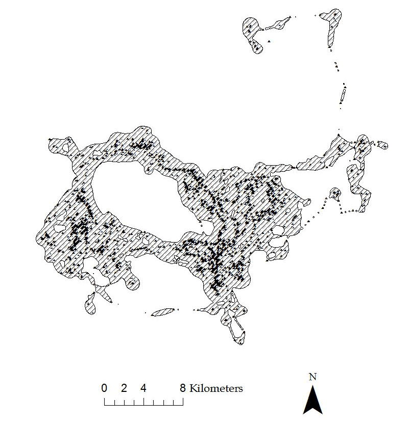
Figure 4.2: Example of 95% BBMM home range for a Florida Panther. - Use brownian.bridge function in package BBMM to run home range
BBMM = brownian.bridge(x=cat143$X, y=cat143$Y, time.lag=cat143$timelag,
location.error=34, cell.size=100)
bbmm.summary(BBMM)
#Plot results for all contours
contours = bbmm.contour(BBMM, levels=c(seq(50, 90, by=10), 95, 99),
locations=cat143, plot=TRUE)
# Print result
print(contours)
NOTE:
(a) Time lag refers to the elapsed time between consecutive GPS locations
that was presented in section 2.3
(b) GPS collar error can be from error reported by the manufacturer of the GPS
collar or from error test conducted at the study site
(c) Cell size refers to grid size we want to estimate the BBMM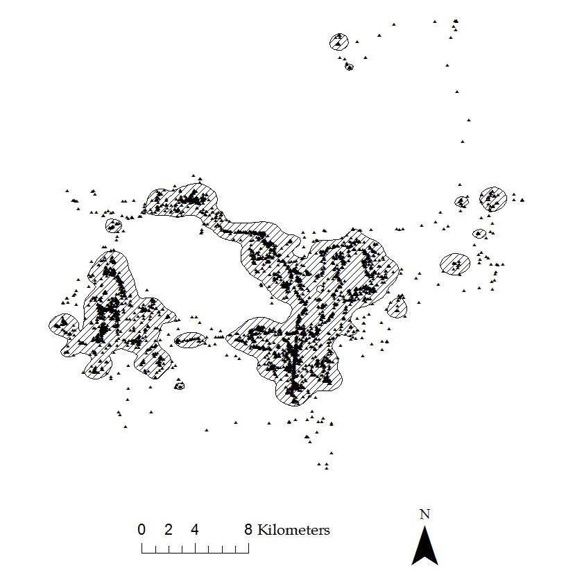
Figure 4.3: Example of 95% KDE home range with hplug-in for a Florida Panther.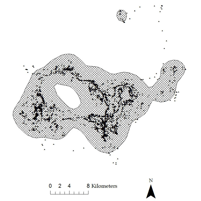
Figure 4.4: Example of 95% KDE home range with href for a Florida Panther.
bbmm.95 = bbmm.95[bbmm.95$probability <= contours$Z[4],] - We need to create output ascii files or shapefiles for graphical representation of size of BBMM (Fig. 4.2). We can also compare BBMM for the Florida panther to KDE using hplug-in (Fig. 4.3) and href (Fig. 4.4). We start by creating a data.frame indicating cells within the contour desired and export as Ascii Grid
bbmm.contour = data.frame(x = BBMM$x, y = BBMM$y, probability = BBMM$probability)
# Pick a contour for export as Asciibbmm.50 = data.frame(x = BBMM$x, y = BBMM$y, probability =
BBMM$probability)
bbmm.50 = bbmm.50[bbmm.50$probability >= contours$Z[1],]
# Output ascii file for cells within specified contour.
m = SpatialPixelsDataFrame(points = bbmm.50[c("x", "y")], data=bbmm.50)
m = as(m, "SpatialGridDataFrame")
writeAsciiGrid(m, "50ContourInOut.asc", attr=ncol(bbmm.50))
# Print result for 80 percent BBMM
print(contours)
# Pick a contour for export as Ascii
bbmm.80 = data.frame(x = BBMM$x, y = BBMM$y, probability =
BBMM$probability)
bbmm.80 = bbmm.80[bbmm.80$probability >= contours$Z[4],]
# Output ascii file for cells within specified contour.
m = SpatialPixelsDataFrame(points = bbmm.80[c("x", "y")], data=bbmm.80)
m = as(m, "SpatialGridDataFrame")
writeAsciiGrid(m, "80ContourInOut.asc", attr=ncol(bbmm.80))
# Print result for 95 percent BBMM
print(contours)
# Pick a contour for export as Ascii
bbmm.95 = data.frame(x = BBMM$x, y = BBMM$y, probability =
BBMM$probability)
bbmm.95 = bbmm.95[bbmm.95$probability >= contours$Z[4],]
# Output ascii file for cells within specified contour.
m = SpatialPixelsDataFrame(points = bbmm.95[c("x", "y")], data=bbmm.95)
m = as(m, "SpatialGridDataFrame")
writeAsciiGrid(m, "95ContourInOut.asc", attr=ncol(bbmm.95))
# Print result for 99 percent BBMM
print(contours)
87
# Pick a contour for export as Ascii
bbmm.99 = data.frame(x = BBMM$x, y = BBMM$y, probability =
BBMM$probability)
bbmm.99 = bbmm.99[bbmm.99$probability >= contours$Z[7],]
# Output ascii file for cells within specified contour.
m = SpatialPixelsDataFrame(points = bbmm.99[c("x", "y")], data=bbmm.99)
m = as(m, "SpatialGridDataFrame")
writeAsciiGrid(m, "99ContourInOut.asc", attr=ncol(bbmm.99))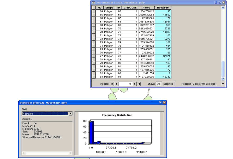
Figure 4.5: This figure shows how to summarize size of home range in ArcMap. -
Now we can create shapefiles of contours from ascii files in ArcMap
(a) Convert ASCII files to Rasters using Conversion Toolbox
Toolbox>Conversion Tools>To Raster>ASCII to Raster
Input ASCII raster file: 50ContourInOut.asc
Output raster: AsciiToRast
Output data type (optional): INTEGER
(b) Convert No Data values to value of 1 and those that are not to value of 0 by:
Toolbox>Spatial Analyst Tools>Math>Logical>Is Null
Input raster: tv53_99contr
Output raster: IsNull_bv53_3
(c) Convert raster probability surface to a shapefile by opening shapefile table.
Highlight all raster cells with a value=1 then open appropriate Toolbox as follows:
Toolbox>Conversion Tools>From Raster>Raster to Polygon
Input raster: IsNull_bv53_3
Field (Optional): Value
Output Polygon Features: RasterT_IsNull_2.shp
Uncheck the "Simplify polygons (optional)" box for proper results. Select OK.
Tool will convert all cells with value=1 to a shapefile with multiple polygons.
(d) Calculate area of new shapefile using appropriate tool (i.e., Xtools) Open table to view area of polygon and summarize to get total size of home range (Fig. 4.5)
Right click on column heading "Hectares"
Select Statistics and Sum will be the total hectares in the home range - Or another way to create shapefiles of contours right in R! There is also an additional way here to create ascii files that will eliminate the need for Step 9 above.
#First an alternate way to create the ascii files after creating "contours" #from Step 5 above.
# Create data.frame indicating cells within the contour desired and export as Ascii Grid
bbmm.contour = data.frame(x = BBMM$x, y = BBMM$y, probability = BBMM$probability)
str(contours) #Look at contour or isopleth levels 1 to 7 (50%-99%)
#$List of 2
#$ Contour: chr [1:7] "50%" "60%" "70%" "80%" ...
#$ Z : num [1:7] 7.35e-05 5.66e-05 4.22e-05 2.81e-05 1.44e-05 .
# Pick a contour for export as Ascii (1 = 50%, 2 = 60%, etc.)
bbmm.50 = bbmm.contour[bbmm.contour$probability >= contours$Z[1],]
bbmm.50$in.out <- 1
bbmm.50 <-bbmm.50[,-3]
# Output ascii file for cells within specified contour.
m50 = SpatialPixelsDataFrame(points = bbmm.50[c("x", "y")], data=bbmm.50)
m50.g = as(m50, "SpatialGridDataFrame")
writeAsciiGrid(m50.g, "50ContourInOut.asc", attr=ncol(bbmm.50)) - Code to start converting the above SpatialPixelsDataFrame to SpatialPolygonsDataFrame and export as ESRI Shapefile
shp.50 <- as(m50, "SpatialPolygonsDataFrame")
map.ps50 <- SpatialPolygons2PolySet(shp.50)
diss.map.50 <- joinPolys(map.ps50, operation = 'UNION')
#Set Projection information
diss.map.50 <- as.PolySet(diss.map.50, projection = 'UTM', zone = '17')
#Re-assign the PolySet to Spatial Polygons and Polygon ID (PID) to 1
diss.map.p50 <- PolySet2SpatialPolygons(diss.map.50, close_polys = TRUE)
data50 <- data.frame(PID = 1)
diss.map.p50 <- SpatialPolygonsDataFrame(diss.map.p50, data = data50) - Use package rgdal to write shapefile to ArcMap
writeOGR(diss.map.p, dsn = ".", layer="contour50", driver = "ESRI Shapefile") - Also use package rgdal to read the shapefile back into R
map.50 <- readOGR(dsn=".", layer="contour50")
plot(map.50) - Repeat steps 8-10 for each contour shapefile desired
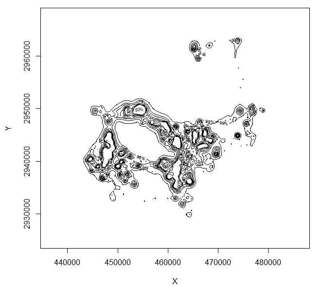
Figure 4.6: Home range of one panther using BBMM showing all contours. -
Another short exercise to subset large dataset by the appropriate time lags in your data but only include locations collected within the 7 hour schedule (i.e., < 421 minutes)
loc <- subset(cat143, cat143$timelag != "NA" & cat143$timelag < 421)
BBMM2 = brownian.bridge(x=loc$X, y=loc$Y, time.lag=loc$timelag, location.error=34,
cell.size=100)
bbmm.summary(BBMM2)
contours1 = bbmm.contour(BBMM2, levels=c(seq(50, 90, by=10), 95, 99),
locations=loc, plot=TRUE)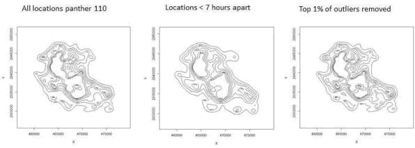
Figure 4.7: Home range using BBMM for panther 110 with various time lags incorporated. -
Or we could exclude the extreme 1% of locations based on a time cutoff that we will determine as in Walter et al. 2011
freq <- as.data.frame(table(round(cat143$timelag)))
#Result is Var1 = the time difference, and Freq = its frequency in the data
freq$percent <- freq$Freq/dim(cat143)[1]*100
freq$sum[1] <- freq$percent[1]
#Loop below runs through data to determine "cutoff" time
for (j in 2:dim(freq)[1]){
freq$sum[j] <- freq$percent[j]+freq$sum[j-1]
}indicator <- which(freq$sum>99)
cutoff <- as.numeric(as.character(freq$Var1[min(indicator)]))
cutoff
# [1] 2939 #2939 minutes -
Need to subset data and only calculate BBMM with timediff < 2940 minutes
loc2 <- subset(loc, loc$timelag < 2940)
str(loc2)
BBMM3 = brownian.bridge(x=loc2$X, y=loc2$Y, time.lag=loc2$timelag, location.error=34,
cell.size=100)
bbmm.summary(BBMM3) -
Plot out resulting home ranges to see differences when altering time difference criteria.
Be sure to change bbmm.contours and rerun Steps 10-11 each time before running each
section of code below
raw.df <- data.frame("x"=cat143$X,"y"=cat143$Y)
##Define the projection of the coordinates
proj4string <- CRS("+proj=utm +zone=17N +ellps=WGS84")
##Make SpatialPointsDataFrame using the XY, attributes, and projection
spdf <- SpatialPointsDataFrame(raw.df, cat143, proj4string = proj4string)
plot(map.99, col="grey",axes=T)
plot(map.95, add=TRUE)
plot(map.90, add=TRUE)
plot(map.80, add=TRUE)
plot(map.50, add=TRUE)
points(spdf)
windows()
loc.df <- data.frame("x"=loc$X,"y"=loc$Y)
##Define the projection of the coordinates
proj4string <- CRS("+proj=utm +zone=17N +ellps=WGS84")
##Make SpatialPointsDataFrame using the XY, attributes, and projection
spdf2 <- SpatialPointsDataFrame(loc.df, loc, proj4string = proj4string)
plot(map.99, col="grey",axes=T)
plot(map.95, add=TRUE)
plot(map.90, add=TRUE)
plot(map.80, add=TRUE)
plot(map.50, add=TRUE)
points(spdf2)

