We are going to focus the remainder of this chapter on Selection Ratios and Resource Selection Functions (RSFs) because Selection Ratios identify a general use of habitat given what is available that can be further explored and studied through use of RSFs. Resource Selection Functions are spatially-explicit models that predict the (relative) probability of use by an animal at a given area/location during a given time, based on the environmental conditions that influence or account for selection. There are numerous types of RSFs that can be performed based on the availability of data collected during the study and there are volumes of literature devoted to the topic of resource selection and sampling designs for radiotelemetry studies (Manly et al. 2002, Cooper and Millspaugh 2001, Erickson et al. 2001, Leban et al. 2001).
Selection Ratio basic functions
widesI may be used to explore resource selection by animals when designs I occur (i.e., habitat use and availability are measured at the population level because individual animals are not identified). The Manly selectivity measure (selection ratio = used/available) is computed and preference/avoidance is tested for each habitat, and the differences between selection ratios are computed and tested (Manly et al. 2002).
widesII computes the selection ratios with design II data (i.e., the same availability for all animals, but use is measured for each one). An example would be to place a minimum convex polygon around all animal locations throughout a study site and define this as "available" to all animals.
widesIII computes the selection ratios for design III data (i.e., use and the availability are measured for each animal with use and availability unique to each individuals movements and habitat use).
Note that all these methods rely on the following hypotheses: (i) independence between animals, and (ii) all animals are selecting habitat in the same way (in addition to "traditional" hypotheses in these kinds of studies: no territoriality, all animals having equal access to all available resource units, etc. (Manly et al. 2002).
- Exercise 8.4 - Download and extract zip folder into your preferred location
- Set working directory to the extracted folder in R under File - Change dir...
-
First we need to load the packages needed for the exercise
library(adehabitatHS) -
Now open the script "MuledeerSR.R" and run code directly from the script
MDsr <- read.csv("MD_winter12.csv",header=T)
#Remove deer that cause errors in plot function later
MDsr <- subset(MDsr,MDsr$animal_id !="647579A")
MDsr$animal_id <- factor(MDsr$animal_id)
used <- subset(MDsr, MDsr$use == 1)
used <- used[c(-1,-3:-6,-8:-15)]
used <- xtabs(~used$animal_id + used$crop, used)
used <- as.data.frame.matrix(used[1:13, 1:5])rand <- subset(MDsr, MDsr$use == 0)
rand <- rand[c(-1,-3:-6,-8:-16)]
rand <- xtabs(~rand$animal_id + rand$crop, rand)
rand <- as.data.frame.matrix(rand[1:13, 1:5])# PVT Code for VegRSF #
pvt.W <- widesIII(used,rand,avknown = FALSE, alpha = 0.1)
pvt.W
par(mfrow=c(1,2))
plot(pvt.W)
#Five categories
#1 = Sunflower,summer crops, random crops, grassland
#2 = Winter crops
#3 = Alfalfa
#4 = Forest
#5 = Shrubland
#Now run on distance to roads binned into 10 categories
MDsr <- read.csv("MD_winter12.csv",header=T)
#Delete deer that have limited data
MDsr <- subset(MDsr,MDsr$animal_id !="647582A" & MDsr$animal_id !="647584A")
MDsr$animal_id <- factor(MDsr$animal_id)
#Bin roads into 4 categories instead of 10
MDsr$NewRoad <- MDsr$BinRoad
levels(MDsr$NewRoad)<-list(class1=c("0-200","200-400"), class2=c("400-600",
"600-800"), class3=c("800-1000","1000-12000","1200-1400"),class4=c("1400-1600",
"1600-1800", "1800-2000"))used <- subset(MDsr, MDsr$use == 1)
used <- used[c(-1:-6,-8:-15)]
used <- xtabs(~used$animal_id + used$NewRoad, used)
used <- as.data.frame.matrix(used[1:12, 1:4])
rand <- subset(MDsr, MDsr$use == 0)
rand <- rand[c(-1:-6,-8:-15)]
rand <- xtabs(~rand$animal_id + rand$NewRoad, rand)
rand <- as.data.frame.matrix(rand[1:12, 1:4])
pvt.road <- widesIII(used,rand,avknown = FALSE, alpha = 0.1)
pvt.road
par(mfrow=c(1,2))
plot(pvt.road)

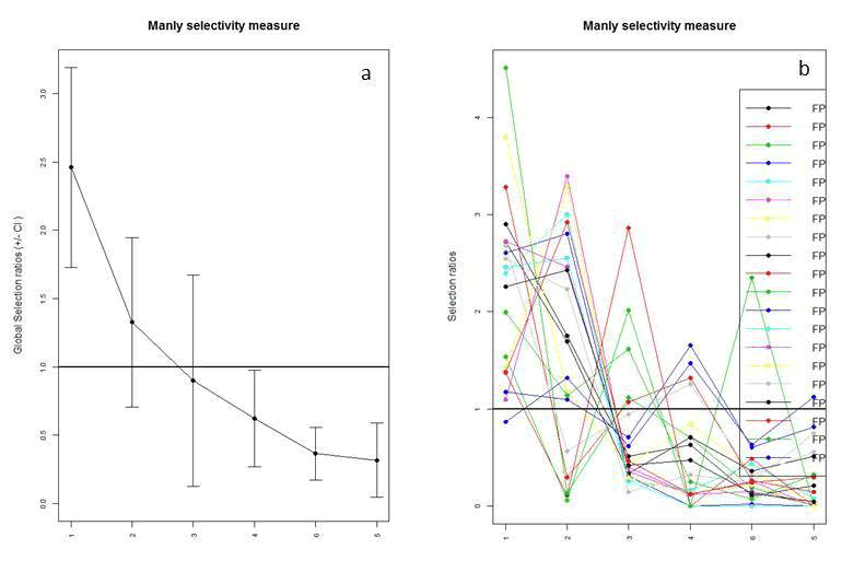
Figure 8.4: Selection ratios for Florida panther for 6 habitat types (1-6) using Manly's Selectivity Measure. Habitat type is on x-axis and selectivity measure is on y-axis for a) all panthers and b) each panther.
Manly's Selectivity Measure in a Design III would suggest that Florida panther are using habitat types 1 and 2 more than they are available (Figure 5.1a). Use of the 6 habitat types for each panther identifies variability between each panther but the trend appears similar across all study animals. Selectivity measure is a general first step look at resource selection but does not really use all the data we have available to use in a Design III study. Although methods of resource selection can be conducted regardless of study design (i.e., I, II, III), the remaining sections of this chapter will focus on Design III because it provides the most detail for each individual animal and should be the goal of most study designs on wildlife for resource selection analysis.

