The first passage time (FPT) is a parameter often used to describe the scale at which patterns occur in a trajectory. For a given scale r, it is defined as the time required by the animals to pass through a circle of radius r. The mean first passage time scales proportionately to the square of the radius of the circle for an uncorrelated random walk (Johnson et al. 1992). Johnson et al. (1992) used this property to differenciate facilitated diffusion and impeded diffusion, according to the value of the coefficient of the linear regression log(FPT) = a * log(radius) + b. Under the hypothesis of a random walk, a should be equal to 2 (higher for impeded diffusion, and lower for facilitated diffusion). Note however, that the value of a converges to 2 only for large values of radius. Another use of the FPT was proposed that, instead of computing the mean of FPT, use the variance of the log(FPT). This variance should be high for scales at which patterns occur in the trajectory, e.g. area restricted search (Fauchald and Tverra 2003). This method is often used to determine the scale at which an animal seaches for food.
The value fpt computes the FPT for each relocation and each radius, and for each animals. This function returns an object of class "fipati", i.e. a list with one component per animal. Each component is a data frame with each column corresponding to a value of radii and each row corresponding to a relocation. An object of class fipati has an attribute named "radii" corresponding to the argument radii of the function fpt. meanfpt and varlogfpt return a data frame giving respectively the mean FPT and the variance of the log(FPT) for each animal (rows) and rach radius (column). These objects also have an attribute "radii".
- Exercise 3.4 - Download and extract zip folder into your preferred location
- Set working directory to the extracted folder in R under File - Change dir...
- First we need to load the packages needed for the exercise
library(adehabitatLT)
library(chron)
library(sp)
library(rgdal) - Now open the script "FPTscript.R" and run code directly from the script
muleys <-read.csv("DCmuleysedited.csv", header=T)
#Code to look at number of relocations per animal
table(muleys$id)
newmuleys <-subset(muleys, muleys$Long > -110.50 & muleys$Lat > 37.3 &
##############################################################################
muleys$Long < -107)
muleys <- newmuleys
## Example of a trajectory of type II (time recorded) ##that must be converted
## to the format POSIX that needs to be done to get proper digits of date for
## use with the adehabitatLT package
##############################################################################
da <- as.character(muleys$GPSFixTime)
da <- as.POSIXct(strptime(muleys$GPSFixTime,format="%Y.%m.%d %H:%M:%S"))
muleys$da <- da - Determine the time difference between each relocation for use later
timediff <- diff(muleys$da)
muleys <-muleys[-1,]
muleys$timediff <-as.numeric(abs(timediff)) - Code to remove known outlier locations if needed
newmuleys <-subset(muleys, muleys$X > 599000 & muleys$X < 705000 & muleys$Y > 4167000 & muleys$timediff < 14401)
muleys <- newmuleys - Create the spatial data from of xy coordinates and additional information
data.xy = muleys[c("X","Y")]
#Creates class Spatial Points for all locations
xysp <- SpatialPoints(data.xy)
#proj4string(xysp) <- CRS("+proj=utm +zone=17 +ellps=WGS84")
#Creates a Spatial Data Frame from
sppt<-data.frame(xysp)
#Creates a spatial data frame of ID
idsp<-data.frame(muleys[2])
#Creates a spatial data frame of dt
dtsp<-data.frame(muleys[24])
#Creates a spatial data frame of Burst
busp<-data.frame(muleys[25])
#Merges ID and Date into the same spatial data frame
merge<-data.frame(idsp,dtsp,busp)
#Adds ID and Date data frame with locations data frame
coordinates(merge)<-sppt
plot(merge)
str(merge) - Create an object of class "ltraj" (i.e., trajectory) for all animals
ltraj <- as.ltraj(coordinates(merge),merge$da,id=merge$id)
plot(ltraj)
#Or we can plot trajectories for each specific animal
plot(ltraj[1])
plot(ltraj[2])
plot(ltraj[3])
plot(ltraj[4])
plot(ltraj[5])
plot(ltraj[6])
plot(ltraj[7]) - Code to plot histograms of distance distribution for each deer
windows()
hist(ltraj[1], "dist", freq = FALSE)
windows()
hist(ltraj[2], "dist", freq = FALSE)
windows()
hist(ltraj[3], "dist", freq = FALSE)
windows()
hist(ltraj[4], "dist", freq = FALSE)
windows()
hist(ltraj[5], "dist", freq = FALSE)
windows()
hist(ltraj[6], "dist", freq = FALSE)
windows()
hist(ltraj[7], "dist", freq = FALSE) - Code below actually creates First Passage Time and mean and variance of fpt
plot(ltraj[1])
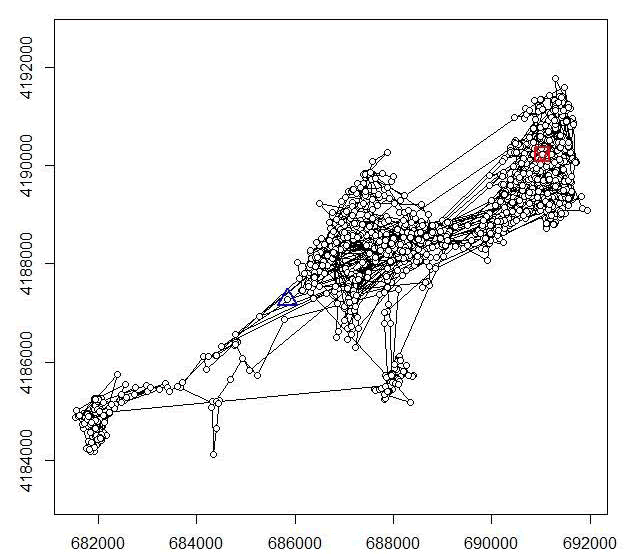
Figure 3.1. Example of a trajectory created using adehabitatLT for a mule deer in Colorado
i1 <- fpt(ltraj[1], seq(300,1000, length=30))
plot(i1, scale = 200, warn = FALSE)
plot(ltraj[2])
i2 <- fpt(ltraj[2], seq(300,1000, length=30))
plot(i2, scale = 500, warn = FALSE)
toto2 <- meanfpt(i2)
toto2
attr(toto2, "radii")
toto2 <- varlogfpt(i2)
toto2
attr(toto2, "radii")
plot(ltraj[3])
i3 <- fpt(ltraj[3], seq(300,1000, length=30))
plot(i3, scale = 500, warn = FALSE)
toto3 <- meanfpt(i3)
toto3
attr(toto3, "radii")
toto3 <- varlogfpt(i3)
toto3
attr(toto3, "radii")
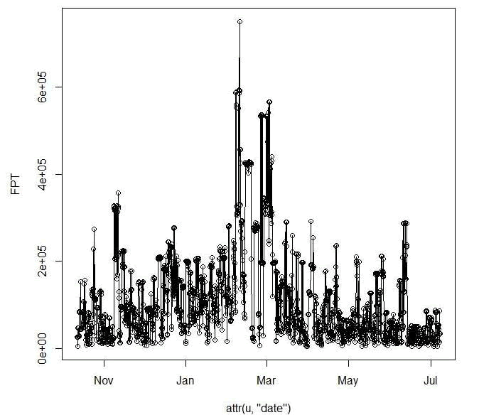
Figure 3.2: Plot of a First Passage Time for a mule deer in Colorado identifying mean FPT by month.
plot(ltraj[4])
i4 <- fpt(ltraj[4], seq(300,1000, length=30))
plot(i4, scale = 500, warn = FALSE)
toto4 <- meanfpt(i4)
toto4
attr(toto4, "radii")
toto4 <- varlogfpt(i4)
toto4
attr(toto4, "radii")
plot(ltraj[5])
i5 <- fpt(ltraj[5], seq(300,1000, length=30))
plot(i5, scale = 500, warn = FALSE)
toto5 <- meanfpt(i5)
toto5
attr(toto5, "radii")
toto5 <- varlogfpt(i5)
toto5
attr(toto5, "radii")
plot(ltraj[6])
i6 <- fpt(ltraj[6], seq(300,1000, length=30))
plot(i6, scale = 500, warn = FALSE)
plot(ltraj[7])
i7 <- fpt(ltraj[7], seq(300,1000, length=30))
plot(i7, scale = 500, warn = FALSE)
toto7 <- meanfpt(i7)
toto7
attr(toto7, "radii")
toto7 <- varlogfpt(i7)
toto7
attr(toto7, "radii")
is.regular(ltraj[1])
plotltr(ltraj[1], "dt")
windows()
plotltr(ltraj[1], "dist")
is.regular(ltraj[2])
plotltr(ltraj[2], "dt")
windows()
plotltr(ltraj[2], "dist")
ltraj[2] - Code to export each trajectory as a shapefile if needed
toto1 <-ltraj2sldf(ltraj[1])
plot(toto1)
writeOGR(toto1,dsn=".",layer="D12", driver = "ESRI Shapefile",overwrite=TRUE)
summary(toto1)
#If we want to define projection before making a shapefile
proj4string <- CRS("+proj=utm +zone=13N +ellps=WGS84")
toto2lines@proj4string <- proj4string
toto2pts@proj4string <- proj4string
#Write lines and points as a shapefile
toto2lines <-ltraj2sldf(ltraj[2],byid=TRUE)
toto2pts <- ltraj2spdf(ltraj[2])
plot(toto2pts)
plot(toto2lines, add=T)
writeOGR(toto2pts,dsn=".",layer="D15pts", driver = "ESRI Shapefile", overwrite_layer=TRUE)
writeOGR(toto2lines, dsn=".", paste("traj_line_",sep=""),driver = "ESRI Shapefile", overwrite=TRUE)
toto3 <-ltraj2sldf(ltraj[3])
plot(toto3)
writeOGR(toto3,dsn=".", layer="D16", driver = "ESRI Shapefile",overwrite=TRUE)
toto4 <-ltraj2sldf(ltraj[4])
plot(toto4)
writeOGR(toto4,dsn=".", layer="D19", driver = "ESRI Shapefile",overwrite=TRUE)
toto5 <-ltraj2sldf(ltraj[5])
plot(toto5)
writeOGR(toto5,dsn=".", layer="D4", driver = "ESRI Shapefile",overwrite=TRUE)
toto6 <-ltraj2sldf(ltraj[6])
plot(toto6)
writeOGR(toto6,dsn=".", layer="D6", driver = "ESRI Shapefile",overwrite=TRUE)
toto7 <-ltraj2sldf(ltraj[7])
plot(toto7)
writeOGR(toto7,dsn=".", layer="D8", driver = "ESRI Shapefile",overwrite=TRUE) - Another look at the time and distance between relocations of each animal. If GPS collars are programmed to collect 1 locations per 24 hours or a location every 4 hours, what would we expect Figure 3.3b to look like? The code can be used to produce these figures and can be used initially to inspect the data if there is concern about consistency in location fixes or distance between each location.
is.regular(ltraj[3])
plotltr(ltraj[3], "dt")
plotltr(ltraj[3], "dist")

