If we want to take both BBMM and KDE to a higher level we can incorporate movement-based estimators of home range. Movement-based Kernel Density Estimation (MKDE) incorporates movements trajectories and habitat components of the landscape your animal occupies (Benhamou 2011, Benhamou and Cornelis 2010). This method requires a habitat layer and the adehabitatHR package requires that no duplicate entries exist for a given date so makes estimates of home range with GPS data problematic. Furthermore, after tirelessly trying this method for days using data with time intervals, we changed to data that had dates but then had to remove duplicates. If you have worked out all of these issues, you can skip ahead to MKDE estimates with your data starting at Step 6.
- Exercise 4.5 - Download and extract zip folder into your preferred location
- Set working directory to the extracted folder in R under File - Change dir...
-
First we need to load the packages needed for the exercise
library(adehabitatHR)
library(adehabitatLT)
library(sp)
library(rgdal)
library(raster)
library(chron)
library(rgeos) - Now open the script "MKDEscript.R" and run code directly from the script
NOTE: Two issues at this step held me back with the method for weeks so we will stress them here:
Extent of the raster layer selected - Although Extent was the lesser problem, it still needs to be address for several reasons. If the extent is too large or raster cell size too small then processing time increases. Although we would not really want to spend the time to clip raster habitat layers for each animal, you may need to have separate rasters for different areas of your study site to cut down on processing time. More importantly, animals need to be within the same grid for analysis using MKDE/BRB home range estimates. This will become more apparent later but preparing habitat or landscape layers for all animals using the same habitat extent will save time in the end.
Projection of the raster layer and locations - Even we missed this one with all ourexperiences and constant issues with data layers in different projections. We assumed that defining the projection with R would take care of this issue but we could not have been more wrong. So before we move forward, we want to demonstrate our thought processes here and how we solved this problem.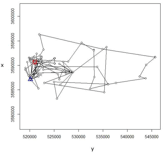
Figure 4.8: Locations of one vulture in UTM 17N.
Using the raster habitat layer that was created using Albers Equal Area Conic similar to exercises from Chapter 1, we can already see the difference in the raster layer by it's orientation and the numbers on the x and y axis are on a different scales compared to the locations in Figure 4.8 (Fig. 4.9).
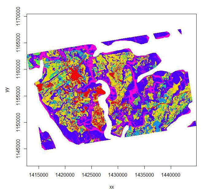
Figure 4.9: Imported habitat layer in Albers Equal Area Conic Projection.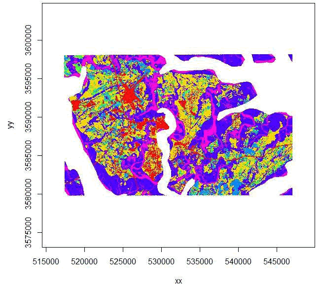
Figure 4.10: Imported habitat layer projected to UTM Zone 17N similar to vulture locations.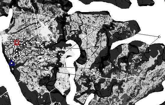
Figure 4.11: Overlay of ltraj on spixdf=habitat in UTM Zone 17N. -
So the raster layer that is included in this exercise is in UTM Zone 17. Now, import the raster layer to have layers in the same projection (Fig. 4.10).
habitat = as(readGDAL("beauzoom100.asc"), "SpatialPixelsDataFrame")
#beauzoom100.asc has GDAL driver AAIGrid
#and has 276 rows and 355 columns
str(habitat)
image(habitat) - Now we need to import our locations and get them in the form we need for this exercise before we can move forward
#Creates a Spatial Points Data Frame for 2 animals by ID
twobirds <-read.csv("Twobirds.csv", header=T)
twobirds$id <-as.factor(twobirds$id)
#Needs to be done to get proper digits of date into R then POSIXct
xtime <- paste(twobirds$OldDate,twobirds$Hour)
twobirds$PosTime <- xtime
#Calculates time difference to use as dt
twobirds$date_time <- chron(as.character(twobirds$OrigDate),twobirds$Hour,
format=c(dates="m/d/y", times="h:m:s"))
timediff <- diff(twobirds$date_time)*24*60
twobirds <-twobirds[-1,]
twobirds$timediff <-as.numeric(abs(timediff))
#Creates class Spatial Points for all locations
data.xy = twobirds[c("x","y")]xysp <- SpatialPoints(data.xy)
#Creates a Spatial Data Frame from
sppt<-data.frame(xysp)
#Creates a spatial data frame of ID
idsp<-data.frame(onebird[2])
#Creates a spatial data frame of Date
datesp<-data.frame(onebird[1])
#Merges ID and Date into the same spatial data frame
merge<-data.frame(idsp,datesp)
#Adds ID and Date data frame with locations data frame
coordinates(merge)<-sppt
proj4string(merge) <- CRS("+proj=utm +zone=17N +ellps=WGS84")
#Cast the Dates as POSIXct dates
merge$DT <-as.POSIXct(strptime(merge$Date, format='%Y%m%d')) - With the same projections for our 2 data layers, we can move forward. First we need to create ltraj as in Chapter 3 and use some additional code to overlay the trajectory onto the Spatial Pixels Data Frame using the command "spixdf" as in the code below that results in Fig. 4.11. Basically, if this works then we are on the right path to moving forward with MKDE.
#Create an ltraj trajectory object.
ltraj <- as.ltraj(coordinates(merge), merge$DT, id = merge$id,
burst = merge$id, typeII = TRUE)
plot(ltraj)
#Code to overlap trajectory onto raster layer
plot(ltraj, spixdf=habitat) - Now identify habitats that can and can not be used by vultures (i.e., water is not used; Fig. 4.12)
#Be sure to do this step after plotting ltraj onto spixdf or won't work!
#This step just builds a "fake" habitat map with habitat=1
fullgrid(habitat) <- TRUE
hab <- habitat
hab[[1]] <- as.numeric(!is.na(hab[[1]]))
image(hab)#See note below
#NOTE: When viewing this image, there may appear to be a periphery of habitat around the extent of the raster that you exported as an ascii from ArcMap. Even deleting the NoData values or categories in ArcMap does not remove this extra data from around the periphy of your habitat layer. To remove this category of data, clip the raster within a boundary box in R or in ArcMap using the following:
Data Management Tools-->Raster-->Raster Dataset-->Copy Raster
Select the optional field in this tool called Ignore Background Value and a related NoData Value field (see help window for more info on how to use these fields).#The step below is needed to convert SpatialGrid to SpatialPixels for use in "ud" estimation (i.e., "habitat" in "grid=habitat" must be of class SpatialPixels
fullgrid(habitat) <- FALSE
class(habitat)#shows it is now class SpatialPixels - Now we can begin to create Movement-based KDEs using biased random bridges (BRBs)
#Assign parameter values for BRB
tmax <- 1*(24*60*60) + 1 ## set the maximum time between locations to be just more
# than 1 day
lmin <- 50 ## locations less than 50 meters apart are considered inactive.
hmin <- 100 ## arbitrarily set to be same as hab grid cell resolution
#Diffusion component for each habitat type using plug-in method
vv<- BRB.D(ltraj, Tmax = tmax, Lmin = lmin, habitat = hab)
vv
vv
$'49'
n D
global 234 146.46958
0 2 24.88662
1 229 140.07425
$'50'
n D
global 272 148.5204
0 0 NaN
1 270 142.3398
attr(,"class")[1] "DBRB"
ud <- BRB(ltraj, D = vv, Tmax = tmax, Lmin = lmin, hmin=hmin, grid = hab, b=TRUE,
extent=0.1, tau = 300)
ud
image(ud)
#Address names in ud by assigning them to be the same as the ids in ltraj
#Must be done before using "getverticeshr" function
names(ud) <- id(ltraj) -
Create contours using getverticeshr to display or export as shapefiles (Fig. 4.15).
ver1_95 <- getverticeshr(ud, percent=95, standardize = TRUE, whi = id(ltraj[1]))
plot(ver1_95)
windows()
ver2_95 <- getverticeshr(ud, percent=95, standardize = TRUE, whi = id(ltraj[2]))
plot(ver2_95) -
Now let's create a new UD using an actual habitat layer that has more than
"used/unused" such as the 7 habitat categories from original dataset
#Start by importing the habitat layer again and run the following
habitat2 = as(readGDAL("beauzoom100.asc"), "SpatialPixelsDataFrame")
plot(ltraj, spixdf=habitat2)
#CODE TO CONDUCT BRB
#Assigne parameter values for BRB
# Parameters for the Biased Random Bridge Kernel approach
tmax <- 1*(24*60*60) + 1 ## set the maximum time between locations to be just
more than 1 day
lmin <- 50 ## locations less than 50 meters apart are considered inactive.
hmin <- 100 ## arbitrarily set to be same as hab grid cell resolution#Diffusion component for each habitat type using plug-in method
vv2 <- BRB.D(ltraj, Tmax = tmax, Lmin = lmin, habitat = habitat2)
vv2
vv2
$'49'
n D
global 234 146.4695789
1 4 1.5909335
2 9 1.5728743
3 0 NaN
4 4 1.2998600
5 1 0.4621171
6 2 0.4812110
7 0 NaN
$'50'
n D
global 272 148.5203800
1 1 1.2267057
2 3 21.6201300
3 0 NaN
4 1 0.7170513
5 0 NaN
6 5 9.5334889
7 0 NaN
98
attr(,"class")
[1] "DBRB"
ud2 <- BRB(ltraj, D = vv2, Tmax = tmax, Lmin = lmin, hmin=hmin, habitat = habitat2,
b=TRUE, extent=0.1, tau = 300, same4all=FALSE)
image(ud2)
names(ud2) <- id(ltraj)
ver1a <- getverticeshr(ud2, percent=95, standardize = TRUE, whi = id(ltraj[1]))
plot(ver1a)
windows()
ver2a <- getverticeshr(ud2, percent=95, standardize = TRUE, whi = id(ltraj[2]))
plot(ver2a) -
Now let's create a new UD witout incorporating an actual habitat layer which reverts to simply KDE with BRB to see if there is difference in the resulting home range shapes
are for each estimate.
#Diffusion component for each habitat type using plug-in method
vv3<- BRB.D(ltraj, Tmax = tmax, Lmin = lmin, habitat = NULL)
vv3
ud3 <- BRB(ltraj, D = vv3, Tmax = tmax, Lmin = lmin, hmin=hmin, habitat = NULL,
b=TRUE, extent=0.1, tau = 300, same4all=FALSE)
image(ud3)
names(ud3) <- id(ltraj)
windows()
ver1b <- getverticeshr(ud3, percent=95, standardize = TRUE, whi = id(ltraj[1]))
plot(ver1b)
windows()
ver2b <- getverticeshr(ud3, percent=95, standardize = TRUE, whi = id(ltraj[2]))
plot(ver2b)

Figure 4.12: Red identifies ocean and tributaries not used by vultures.
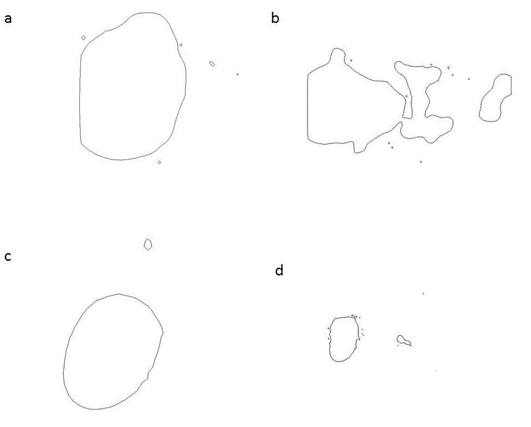
Figure 4.13: Contours of home range for 2 black vultures estimated using the Movement-based kernel density method (MKDE)

