- Exercise 3.5 - Download and extract zip folder into your preferred location
- Set working directory to the extracted folder in R under File - Change dir...
-
First we need to load the packages needed for the exercise
library(adehabitatLT)
library(chron)
library(raster)
library(sp) - Now open the script "RegTrajScript.R" and run code directly from the script
muleys <-read.csv("DCmuleysedited.csv", header=T)
str(muleys) #CODE TO SUBSET FOR AN INDIVIDUAL ANIMAL
muley15 <- subset(muleys, id=="D15")
str(muley15)
summary <- table(muley15$UTM_Zone,muley15$id)
summary
muley15$id
#muley15$DT <-as.POSIXct(strptime(muley15$GPSFixTime, format='%Y.%m.%d %H:%M:%OS'))
#muley15$DT
#Sort data to address error in code
muley15 <- muley15[order(muley15$GPSFixTime),]
muley15[1:10,]#code displays the first 10 records to look at what sorting did to data
str(muley15)
######################################################
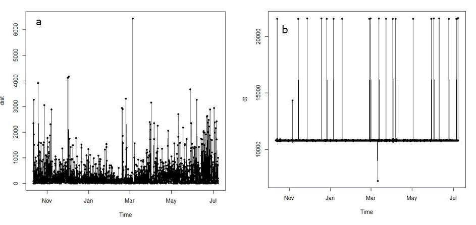
## Example of a trajectory of type II (time recorded) Figure 3.3: Summaries of distance and time (dt) between relocations for mule deer D16.
### Conversion of the date to the format POSIX. Needs to be done to get proper #digits of date into R then POSIXct
library(chron)
da <- as.character(muley15$GPSFixTime)
da <- as.POSIXct(strptime(muley15$GPSFixTime,format="%Y.%m.%d %H:%M:%S"))
muley15$da <- da
timediff <- diff(muley15$da)
muley15 <-muley15[-1,]
muley15$timediff <-as.numeric(abs(timediff))
str(muley15)
newmuleys <-subset(muley15, muley15$X > 599000 & muley15$X < 705000 & muley15$Y > 4167000 & muley15$timediff < 14401)
muley15 <- newmuleys
data.xy = muley15[c("X","Y")]
#Creates class Spatial Points for all locations
xysp <- SpatialPoints(data.xy)
#proj4string(xysp) <- CRS("+proj=utm +zone=17 +ellps=WGS84")
#Creates a Spatial Data Frame from
sppt<-data.frame(xysp)
#Creates a spatial data frame of ID
idsp<-data.frame(muley15[2])
#Creates a spatial data frame of dt
dtsp<-data.frame(muley15[24])
#Creates a spatial data frame of Burst
busp<-data.frame(muley15[23])
#Merges ID and Date into the same spatial data frame
merge<-data.frame(idsp,dtsp,busp)
#Adds ID and Date data frame with locations data frame
coordinates(merge)<-sppt
plot(merge)
str(merge)
### Creation of an object of class "ltraj"
ltraj <- as.ltraj(coordinates(merge),merge$da,id=merge$id)
plot(ltraj)
ltraj
#CAN BE USED TO REMOVE TIME FROM DATE IN GPSFIXTIME COLUMN
#Date <- as.character(muleys$GPSFixTime)
#Date <- as.POSIXct(strptime(muleys$GPSFixTime,"%Y.%m.%d"))
#muleys$Date <- Date
#str(muleys)
#We want to study the trajectory of the day at the scale of the day. We define #one trajectory per day. The trajectory should begin at 22H00. The following function returns TRUE if #the date is comprised between 06H00 and 23H00 (i.e. results in 3 locations/day bursts)
foo <- function(date) {
da <- as.POSIXlt(date)
ho <- da$hour + da$min
return(ho>15.9&ho<23.9)
}
deer <- cutltraj(ltraj, "foo(date)", nextr = TRUE)
deerz
#Remove the first and last burst if needed?
#deer2 <- deer[-c(1,length(deer))]
#bind the trajectories
deer3 <- bindltraj(deer)
deer3
plot(deer3)
is.regular(deer)
FALSE
plotltr(deer3, "dist")
#The relocations have been collected every 3 hours, and there are some missing #data.
## The reference date: the hour should be exact (i.e. minutes=0):
refda <- strptime("00:00", "%H:%M")
refda
#Set the missing values
deerset <- setNA(deer3, refda, 3, units = "hour")
#Now, look at dt for the bursts:
plotltr(deerset, "dt")
#dt is nearly regular: round the date:
deerset1 <- sett0(deerset, refda, 3, units = "hour")
plotltr(deerset1, "dt")
is.regular(deerset1)
#Deerset1 is now regular
##Is the resulting object "sd" ?
is.sd(deerset1)
#Show the changes in the distance between successive relocations with the time
windows()
plotltr(deerset1, "dist")
## Segmentation of the trajectory based on these distances
lav <- lavielle(deerset1, Lmin=2, Kmax=20)
## Choose the number of segments
chooseseg(lav)
## 20 segments seem a good choice
## Show the partition
kk <- findpath(lav, 20)
kk
##Results of code
*********** List of class ltraj ***********
#Type of the traject: Type II (time recorded)
#Regular traject. Time lag between two locs: 10800 seconds
#Characteristics of the bursts:
# id burst nb.reloc NAs date.begin date.end #1 D15 Segment.1 199 27 2011-10-12 04:00:00 2011-11-05 22:00:00 #2 D15 Segment.2 2 0 2011-11-06 01:00:00 2011-11-06 03:00:00 #3 D15 Segment.3 455 64 2011-11-06 06:00:00 2012-01-02 00:00:00 #4 D15 Segment.4 1 0 2012-01-02 03:00:00 2012-01-02 03:00:00 #5 D15 Segment.5 2 0 2012-01-02 06:00:00 2012-01-02 09:00:00 #6 D15 Segment.6 1 0 2012-01-02 12:00:00 2012-01-02 12:00:00 #7 D15 Segment.7 64 8 2012-01-02 15:00:00 2012-01-10 12:00:00 #8 D15 Segment.8 3 1 2012-01-10 15:00:00 2012-01-10 21:00:00 #9 D15 Segment.9 2 0 2012-01-11 00:00:00 2012-01-11 03:00:00 #10 D15 Segment.10 33 4 2012-01-11 06:00:00 2012-01-15 06:00:00 #11 D15 Segment.11 5 1 2012-01-15 09:00:00 2012-01-15 21:00:00 #12 D15 Segment.12 3 0 2012-01-16 00:00:00 2012-01-16 06:00:00 #13 D15 Segment.13 2 0 2012-01-16 09:00:00 2012-01-16 12:00:00 #14 D15 Segment.14 336 46 2012-01-16 15:00:00 2012-02-27 12:00:00 #15 D15 Segment.15 4 1 2012-02-27 15:00:00 2012-02-28 00:00:00 #16 D15 Segment.16 250 35 2012-02-28 03:00:00 2012-03-30 07:00:00 #17 D15 Segment.17 1 0 2012-03-30 10:00:00 2012-03-30 10:00:00 #18 D15 Segment.18 5 2 2012-03-30 13:00:00 2012-03-31 01:00:00 #19 D15 Segment.19 1164 154 2012-03-31 04:00:00 2012-08-23 13:00:00 #20 D15 Segment.20 63 9 2012-08-23 16:00:00 2012-08-31 10:00:00
#Notice that the results show for each burst:
(1) number of relocations
(2) number of relocations removed (i.e., NA)
(3) begin and end dates
#Now if we reduce the number of segments we get the following bursts:
## Segmentation of the trajectory based on these distances
lav <- lavielle(deerset1, Lmin=2, Kmax=10)
## Choose the number of segments
chooseseg(lav)
## 20 segments seem a good choice
##Show the partition
k <- findpath(lav, 10)
kk
*********** List of class ltraj ***********
#Type of the traject: Type II (time recorded)
#Regular traject. Time lag between two locs: 10800 seconds
#Characteristics of the bursts:
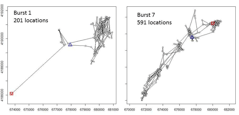
# id burst nb.reloc NAs date.begin date.end #1 D15 Segment.1 201 27 2011-10-12 04:00:00 2011-11-06 03:00:00 #2 D15 Segment.2 456 64 2011-11-06 06:00:00 2012-01-02 03:00:00 #3 D15 Segment.3 2 0 2012-01-02 06:00:00 2012-01-02 09:00:00 #4 D15 Segment.4 1 0 2012-01-02 12:00:00 2012-01-02 12:00:00 #5 D15 Segment.5 102 13 2012-01-02 15:00:00 2012-01-15 06:00:00 #6 D15 Segment.6 10 1 2012-01-15 09:00:00 2012-01-16 12:00:00 #7 D15 Segment.7 591 82 2012-01-16 15:00:00 2012-03-30 10:00:00 #8 D15 Segment.8 5 2 2012-03-30 13:00:00 2012-03-31 01:00:00 #9 D15 Segment.9 1164 154 2012-03-31 04:00:00 2012-08-23 13:00:00 #10 D15 Segment.10 63 9 2012-08-23 16:00:00 2012-08-31 10:00:00
#We can look at each segment to inspect the path traveled during the burst:
plot(kk[1])
plot(kk[2])
plot(kk[3])
plot(kk[6])
plot(kk[7])
plot(kk[9])

Figure 3.4: Bursts of movements for mule deer D15 after creating segements based for focal use areas.

