Transformations in ArcMap can be the most troublesome component of spatial analysis that is often overlooked as the reason for errors in data analysis. We will briefly go into the 2 most common problems requiring our assistance from collaborators and potential solutions.
1. What coordinate system were the data collected in?
It seems that every GPS collar, handheld GPS unit, GIS landcover layer, etc. has been created using a different coordinate system and it's not the one you have at your study site. Or perhaps NAD 1927 was used and you decided to be modern and want to use NAD 1983. Regardless, the coordinate systems must match even though ArcMap often overlays them with "on the fly projections". The "on the fly" component of ArcMap is great for visualization but not for spatial ecologists that need data analysis. We often can determine which coordinate system the data were created in using the metadata to define a coordinate system or project the data into a coordinate system for data analysis.
2. A Toolbox in ArcMap may not extract data or clip data properly
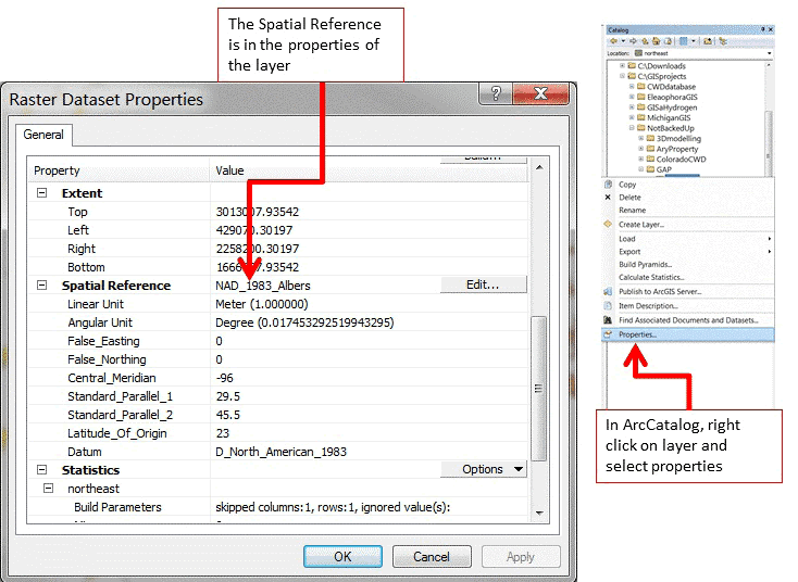
As mentioned previously, data collected with a GPS collar or handheld GPS may not be in the same geographic or projected coordinate system as the GIS layers you download or receive from collaborators (i.e., Digital Elevation Data, National Land Cover Data; Fig. 1.3). As you attempt to use a Toolbox function, such as clipping National Land Cover Data within the extent of your GPS locations, an error may result.

Figure 1.3: How to find coordinates system of GIS layer in ArcCatalog or Table of Contents in ArcMap
We will now explore some transformations of data in R to help understand what Projections and Transformations are all about. The dataset that follows is for a project in Colorado with mule deer equipped with GPS collars that collected locations every 3 hours. The purpose of the study was to determine mule deer use of agricultural crops, sunflowers in this case, in response to years of damage complaints from farmers. We will use this subset of dataset in later exercises as well.
- Exercise 1.4 - Download and extract zip folder into your preferred location
- Set working directory to the extracted folder in R under File - Change dir...
- First we need to load the packages needed for the exercise
library(rgdal) - Now open the script "MDprojections.R" and run code directly from the script
study.states<-readOGR(dsn=".",layer="MDcounties")
#OGR data source with driver: ESRI Shapefile
#Source: ".", layer: "MDcounties"
#with 38 features and 8 fields
#Feature type: wkbPolygon with 2 dimensions
plot(study.states, col="grey")
#Let's zoom into the region we have locations instead of county level
study.zoom<-readOGR(dsn=".",layer="MDzoom")
OGR data source with driver: ESRI Shapefile
Source: ".", layer: "MDzoom"
with 1 features and 1 fields
Feature type: wkbPolygon with 2 dimensions
plot(study.zoom, col="grey") - Import the csv file that contains all the mule deer locations by ID
muleys <-read.csv("muleysexample.csv", header=T)
str(muleys) - Create a spatial data frame of raw mule deer locations with projection defined similar to study site shapefile (i.e., WGS84)
coords<-data.frame(x = muleys$Long, y = muleys$Lat)
crs<-"+proj=longlat +ellps=WGS84 +datum=WGS84 +no_defs +towgs84=0,0,0"
coords
plot(coords) - Remove outlier locations
newmuleys <-subset(muleys, muleys$Long > -110.50 & muleys$Lat > 37.3
& muleys$Long < -107)
muleys <- newmuleys - Create a new spatial data frame of mule deer locations with outliers removed and projection defined similar to study site shapefile (i.e., WGS84)
coords<-data.frame(x = muleys$Long, y = muleys$Lat)
crs<-"+proj=longlat +ellps=WGS84 +datum=WGS84 +no_defs +towgs84=0,0,0"
coords
plot(coords) - Create a spatial points data frame of mule deer locations projection defined similar to study site shapefile (i.e., WGS84)
deer.spdf <- SpatialPointsDataFrame(coords= coords, data = muleys, proj4string = CRS(crs))
deer.spdf[1:5,]
class(deer.spdf)
proj4string(deer.spdf)
points(deer.spdf)
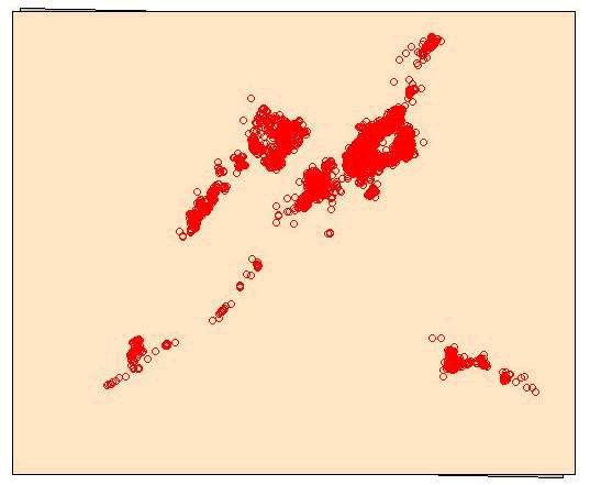
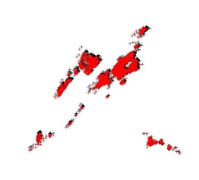
points(deer.spdf, col="yellow") - Now let's project both the mule deer locations and study site shapefile to NAD83 UTM Zone 12 (Fig. 1.4, 1.5)
new.crs <-CRS("+proj=utm +zone=12 +datum=WGS84")
MDzoomUTM12 <-spTransform(study.zoom, CRS=new.crs)
par(new=TRUE)
plot(MDzoomUTM12, col="bisque")
class(MDzoomUTM12)
proj4string(MDzoomUTM12)
summary(MDzoomUTM12)
#projection for mule deer locations
deer.crs <-CRS("+proj=utm +zone=12 +datum=WGS84")
deerUTM12 <-spTransform(deer.spdf, CRS=deer.crs)
points(deerUTM12, col="red")
class(deerUTM12)
proj4string(deerUTM12)
deerUTM12[1:5,]
#See new projected coordinates in UTM 12N for the first 5 locations
coordinates(deerUTM12)[1:5,]
x y

Figure 1.4: Study area projected into UTM Zone 12N with original WGS84 underneath
[1,] 677825.2 4192832
[2,] 677853.8 4192787
[3,] 677736.3 4192728
[4,] 677595.9 4192398
[5,] 677666.2 4192362
#plot coordinates in Lat Long over coordinates in UTM 12N
plot(coords)
par(new=TRUE)
plot(deerUTM12, col="red")
windows()
plot(study.zoom)
par(new=TRUE)
plot(deer.spdf, col="red")
windows()
plot(MDzoomUTM12,col="bisque")
par(new=TRUE)
plot(deerUTM12, col="red")
#another method to project data
require(rgdal)
make_EPSG()
nad83 <-EPSG[grep("NAD83",EPSG$note),]
nad83[grep("UTM zone 12N", nad83$note),]

Figure 1.5: Mule deer locations projected into UTM Zone 12N (red) with original locations in
WGS84 (black)

