4.8 Local Convex Hull (LoCoH)

Local convex hull nonparametric kernel method (LoCoH), which generalizes the minimum convex polygon method, produces bounded home ranges and better convergence properties than parametric kernel methods as sample size increases (Getz et al. 2007, Getz and Wilmers 2004). The use of LoCoH also has been investigated for identifying hard boundaries (i.e. rivers, canyons) of home ranges because it is essentially a non-parametric kernel method using minimum convex polygon construction. The use of polygons instead of kernels gives LoCoH the ability to produced hard edges or boundaries that will not overlap into unused spaces common to kernel methods (Getz et al. 2007). Without getting into to much detail, LoCoH has 3 modifications that reference the k-nearest neighbor convex hulls (NNCH) in some form. The 3 terms are fixed k, fixed radius (r-NNCH), and adaptive (a-NNCH) that are comparable to kernel smoothing of href, lscv, and plug-in, respectively.

1. Exercise 4.8a - Download and extract zip folder into your preferred location
2. Set working directory to the extracted folder in R under File - Change dir...

3. First we need to load the packages needed for the exercise
   library(adehabitatLT)
   library(move)
   library(circular)
   library(sp)

4. Now open the script "LocohGUIscript.R" and run code directly from the script
5. We will begin using LoCoH by first downloading the proper script NNCH.R
   
   NOTE: LoCoH GUI will not work in earlier versions of R with adehabitat in Windows 10 but worked with Windows Vista so may need to download most recent version of R along with package adehabitatHR.
6. Then install the script to use with the adehabitatHR package:
   
   source("NNCH.R")
   
   
7. Next we need to install the graphic user interface locoh_gui.R
   
   source("locoh_gui.R")
   
   
8. To access the GUI we can simply invoke LoCoH using the command
   
   locoh()
   
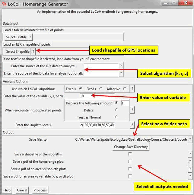
   The LoCoH GUI will pop up in a separate window in R (Fig. 4.15). Refer to adehabitatHR manual and Getz et al. (2007) for more details on LoCoH inputs.
   
   
9. Then browse for the appropriate shapefile of animal locations (Fig. 4.15)
   
   
10. Choose the algorithm (k, r, a) and enter the value of the variable (Fig. 4.15)
    
    
11. Select the option that is appropriate for handling duplicate points (Fig. 4.15)
12. Save resulting home range as shapefiles or pdfs (Fig. 4.15)

Figure 4.15: The LoCoH GUI.

Alternatively, for the purists that don't like GUIs or need estimates of home range for multiple animals we can calculate LoCoH directly in R using the original adehabitat package (Calenge 2007) which is not recommended and removed from a previous version of this manual. We can use the adehabitatHR package to estimate LoCoH with any of the 3 algorithms (i.e., k, r, adaptive):

1. Exercise 4.8b - Download and extract zip folder into your preferred location
2. Set working directory to the extracted folder in R under File - Change dir...

3. First we need to load the packages needed for the exercise
   library(adehabitatHR)
   library(shapefiles)
   library(rgeos)
   library(rgdal)
   library(maptools)

4. Now open the script "CodeHRscript.R" and run code directly from the script

   panther <- read.csv("pantherjitter2.csv")
   str(panther)
   panther$CatID <- as.factor(panther$CatID)
   #Or explore with one panther with 381 relocations
   cat159 <- subset(panther, CatID=="159")
   str(cat159)

   cat159$CatID <- factor(cat159$CatID)
   #Get the relocation data from the source file
   data.xy = cat159[c("x","y")]
   xysp <- SpatialPoints(data.xy)
   #Creates a Spatial Data Frame from
   sppt<-data.frame(xysp)
   #Creates a spatial data frame of ID
   idsp<-data.frame(cat159[1])
   #Adds ID and Date data frame with locations data frame
   coordinates(idsp)<-sppt
   proj4string(idsp) <- CRS("+proj=utm +zone=17 +ellps=WGS84")
   locsdf <-as.data.frame(idsp)
   head(locsdf)
   ## Shows the relocations
   plot(data.xy, as.numeric(locsdf[,1]), col="red")
   ## Examines the changes in home-range size for various values of k
   ## Be patient! the algorithm can be very long
   ar <- LoCoH.k.area(idsp, k=c(16:25))
   ## 24 points seems to be a good choice (rough asymptote for all animals)
   ## the k-LoCoH method:
   nn <- LoCoH.k(idsp, k=24)
   ## Graphical display of the results
   plot(nn, border=NA)
   ## the object nn is a list of objects of class
   ## SpatialPolygonsDataFrame
   length(nn)
   names(nn)
   class(nn[[1]])
   ## shows the content of the object for the first animal
   as.data.frame(nn[[1]])
   ## The 95% home range is the smallest area for which the
   ## proportion of relocations included is larger or equal
   ## to 95% In this case, it is the 339th row of the
   ## SpatialPolygonsDataFrame.
   ## The area covered by the home range panther 159
   ## is equal to 5506.04 ha.
   ## shows this area:
   plot(nn[[1]][339,], lwd=2)
   #The 50% home range code is on line 146
   plot(nn[[1]][146,], add=TRUE)
   #The 99% home range code is on line 133
   plot(nn[[1]][363,], lwd=3, add=TRUE)
   ##We can write shapefiles for specific sizes of home range
   ver <-getverticeshr(nn)

   ver
   plot(ver)
   writeOGR(ver,dsn="FixedK",layer="FixedK24", driver = "ESRI Shapefile",
   overwrite=TRUE)
   ##Or we can write shapefiles for specific sizes of home range but overwrite will not work so must edit path so "FixedK" folder is created with code below.
   ver50 <-getverticeshr(nn, percent=50)
   writeOGR(ver50,dsn="FixedK",layer="50FixedK24", driver = "ESRI Shapefile", overwrite=TRUE)
   ver95 <-getverticeshr(nn, percent=95)
   writeOGR(ver95,dsn="FixedK",layer="95FixedK24", driver = "ESRI Shapefile", overwrite=TRUE)
   ver99 <-getverticeshr(nn, percent=99)
   writeOGR(ver99,dsn="FixedK",layer="99FixedK24", driver = "ESRI Shapefile", overwrite=TRUE)