1.6 Manipulate Polygon Layer

1. Exercise 1.6 - Download and extract zip folder into your preferred location
2. Set working directory to the extracted folder in R under File - Change dir...
3. First we need to load the packages needed for the exercise
   
   library(rgdal)
   library(maptools)
   library(foreign)
4. Now open the script "SoilScript.R" and run code directly from the script
   
   soils<-readOGR(dsn=".",layer="Soil_Properties")
   soils@proj4string ###get projection
   plot(soils)
   names(soils) ###get attribute data
   
   #Rename ArcMap category headings to something more familiar
   soils$Clay <- soils$SdvOutpu_1
   soils$pH <- soils$SdvOutpu_2
   soils$CEC <- soils$SdvOutpu_3
   
   #Shapefiles contain several slots which can be called with the "@" symbol
   #or slot(object, "data")
   
   soils@data #= a data frame with n observations associated with X covariates,
   soils@polygons #=the number of polygons that the shapefile consists of
   soils@plotOrder #= the order of the polygons
   soils@bbox #= boundary box
   soils@proj4string #= projection
   #Within the slot
   soils@polygons [[1]] ###will bring up the first polygon
   soils@polygons [[1]]@area ###will bring up the area for the first polygon
   soils@polygons[[1]]@ID ##will retrieve the ID of the first polygon
   soils@polygons[[1]]@plotOrder ##will retrieve the order of the first polygon
5. Select portions of the data that fit some set criteria
   
   ##Highlights the areas that Percent Clay polygons are over 30%
   plot(soils, col=grey(1-soils$Clay > 30))
   plot(soils)
   high.clay<- soils[soils$Clay>30,]
   plot(high.clay, border="red", add=TRUE)
   
   ##Highlights the areas that Cation Exchange Capacity is greater than 14
   high.CEC<- soils[soils$CEC>14,]
   plot(high.CEC, border="green", add=TRUE)
   
   ##Highlights the areas that soil pH is greater than 8
   high.pH <- soils[soils$pH>8,]
   plot(high.pH, border="yellow", add=TRUE)
6. Bring in locations of harvested mule deer
   
   #Import mule deer locations from harvested animals tested for CWD
   
   mule <-read.csv("MDclip.csv", header=T)
   str(mule)
   coords<-data.frame(x = mule$x, y = mule$y)
   crs<-"+proj=utm +zone=13 +datum=WGS84 +no_defs +towgs84=0,0,0"
   coords
   
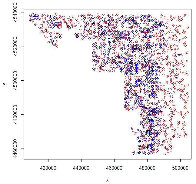
   plot(coords, col="blue")
   par(new=TRUE)
7. Let's generate random points with the extent of the soil layer
   
   #Sampling points in a Spatial Object### will give a regular grid
   samples<-spsample(soils, n=1000, )
   samples@proj4string
   
   #Plot them to see if it worked or to create output figures
   plot(soils, col="wheat")
   points(coords, col="blue")
   points(samples, col="red")
8. Creates a SpatialPoints object from the location coordinates
   
   samples@bbox <- soils@bbox
   samples@proj4string <- soils@proj4string
9. Extract and tally Clay soil types for random samples and mule deer locations:
   
   #Match points with soil polygons they occur in
   soils.idx<- over(samples,soils)
   locs <- SpatialPoints(coords)
   locs@proj4string <- soils@proj4string
   soils.locs<- over(locs, soils)
   
   #Tally clay soil types for random samples
   obs.tbl <- table(soils.idx$Clay[soils.idx$Clay])
   obs.tbl
   
   #Also tally soil types for each mule deer sampled
   obs.tbl2 <- table(soils.locs$Clay[soils.locs$Clay])
   obs.tbl2
10. Convert the counts to proportions:
    
    obs <- obs.tbl/sum(obs.tbl)
    obs
    
    obs2 <- obs.tbl2/sum(obs.tbl2)
    bs2

Figure 1.6 Overlay of mule deer locations with random locations generated in R